LEFT and RIGHT
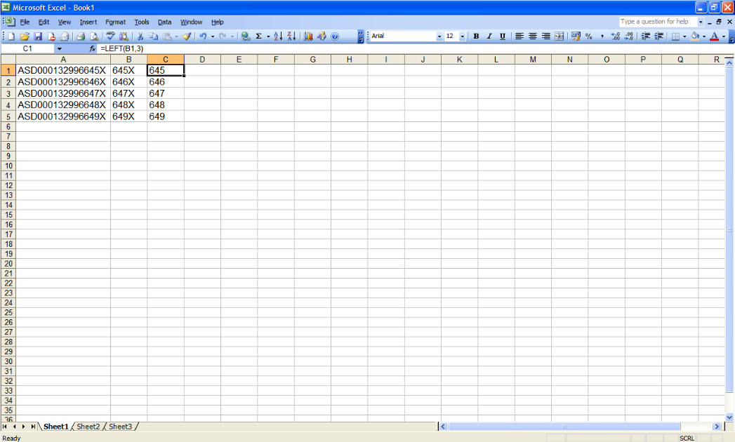
You probably won’t use LEFT and RIGHT very often, but they can save a huge amount of time. Imagine you have a list of product codes, but they have a standard set of letters before and after the bit you’re interested in. Something like this:
ASD000132996645X
ASD000132996646X
ASD000132996647X
ASD000132996648X
ASD000132996649X
It would be much easier to work with the list if you didn’t have all those unnecessary letters and numbers. That’s where these Functions come in.
The basic formula is:
=RIGHT(cell reference,no. chars)
Just replace the words ‘cell reference’ with the reference of the cell you want to include, and ‘no. chars’ with the number of characters you want to include from that direction. If you’re using RIGHT count from the right, if you’re using LEFT count from there. Easy! So for example, in our case it might be:
=RIGHT(A1,4)
Assuming that our list started from the top of column A, this would return ‘645X’, because those are the first 4 characters if you read from the right-hand side of the cell.
So what if we want to remove the X from the end of the code? Easy, just use the other function! If the first Excel formula went next to the first code, in cell B1, the next formula would look like this:
=LEFT(B1,3)
Notice how we’re targeting B1 instead of A1? That’s because in this case we need 2 Excel formulas to get the result we want. There are ways around this, but for now let’s keep it basic.
The second formula will return the result we wanted: ‘645’.

I hope you've found this page useful; I’d appreciate it if you’d take the time to let me know how you rate it.
If you’re still struggling with the LEFT and RIGHT Functions you might find it helpful to have another look at the Getting started with Excel formulas page.
Looking for more? Return to Excel Formulas or the Office Software homepage


