Formatting in Excel

Formatting in Excel is easy, but is often overlooked. It’s really important that you use formatting to make your spreadsheets easier to use. Whether you’re going to present information to other people, you’re sharing a spreadsheet with others or even if it’s just for yourself: Formatting is important.

Fortunately it's also easy!

Please don’t misunderstand, the purpose of formatting isn’t usually to make your spreadsheet pretty – It’s to make it more intuitive.

For example, which of these tables is easier to understand at a glance?

Number 1 -

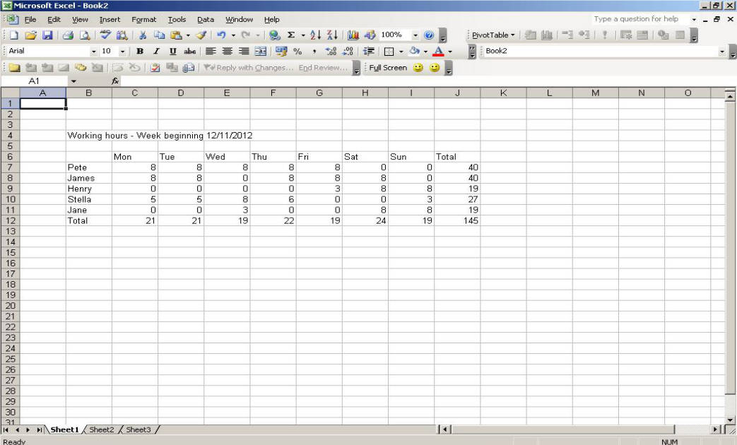
Or number 2 -

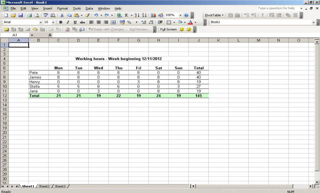
Not a difficult question, I think, so let’s get started.

Column widths and Row heights

You’ll often find that you need to alter the layout of your rows and columns – Fortunately this is very easy.

If you want to manually alter the layout of a row or column just hover your mouse cursor over the right-hand side of the column label or bottom of the row label, hold down the left mouse button and drag it to the size you want:

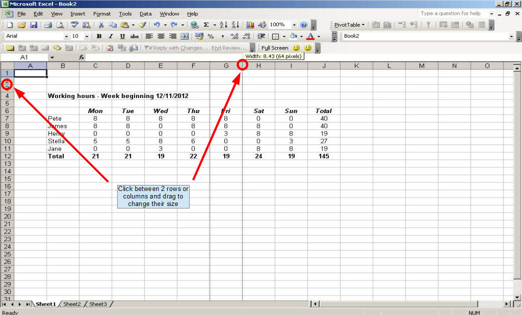
Alternatively you can have Excel automatically resize a column or row to the minimum size required to fit the contents of its cells. To do this just double click on the right-hand side of the column label or the bottom of the row label.

You can apply either of these techniques to groups of columns or rows by selecting a group of them and then performing the actions listed above to just one of them. This will automatically make the same changes to the whole group.

Fonts and font sizes

This is the simplest form of formatting in Excel – There really isn’t any need to change away from the default font for the vast majority of the time. The default font in Excel is Arial which is a sans-serif font. It’s usually best to stick with sans serif fonts for spreadsheets because they’re easy to read - Arial and Verdana are good choices.

If you do want to change the font or size of font that you’re using, just select the cells you want to change and use the formatting toolbar:

If you’re using Office 2007 or 2010 you can find the formatting toolbar in the Home section of the ribbon at the top of the screen.

Text Formatting - Bold, Italic and Underline

Bold, Italic and Underline are great ways to draw attention to text in certain cells. As a general rule you probably won’t want to use Underline very often in spreadsheets, but by all means use it if you think it’ll be helpful to your target audience.

Bold and Italic are a good way to draw attention to column and row headings or labels. For example if we return to our example, just making some of the fields bold instantly makes it much easier to understand:

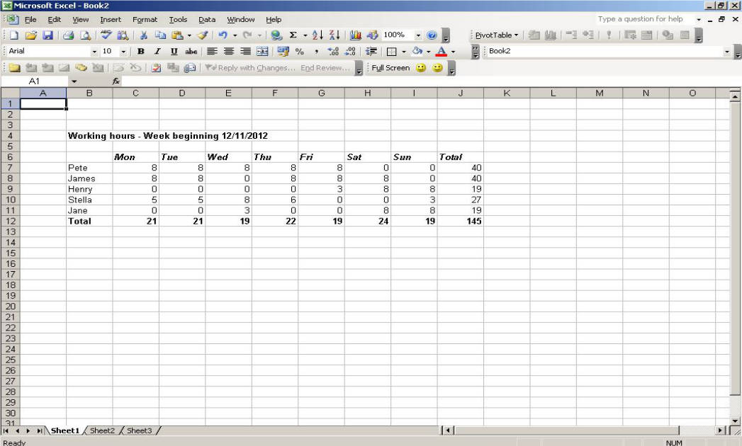
Again these features are easy to use, juts highlight the cells you want to change and use the formatting toolbar to make the contents Bold, Italic or Underlined.

If you’re using Office 2007 or 2010 you can find the formatting toolbar in the Home section of the ribbon at the top of the screen.

The last button in this toolbar is called Strikethrough – It’s very rarely used, but it can sometimes be useful, e.g. for electronic to-do lists.

If you’re wondering, it makes text look like this.

Alignment

Alignment is another great way to neaten up your spreadsheets. By default Excel will align text to the left-hand side of a cell, and numbers to the right-hand side. That's fine for the most part, but it looks much nicer if your headings are center aligned. For example:

I’ve chosen to center the table contents as well as the column headings – That’s a personal preference. It doesn’t make a huge amount of difference when you’re working in Excel, but I’ve found that it’s easier to read tables when they’re printed out of the contents are center aligned.

Again, all you need to do is highlight the cells you want to alter and use the formatting toolbar to align them to the right, left or center.

Orientation

Now it’s time to introduce yourself to a different way of formatting cells. Right click on a cell and select ‘Format Cells’ from the drop-down menu. Don’t worry about all the options for now, just select the alignment tab. The exact layout of the menu will differ depending on the version of Excel that you’re using, but it will look pretty much like this:

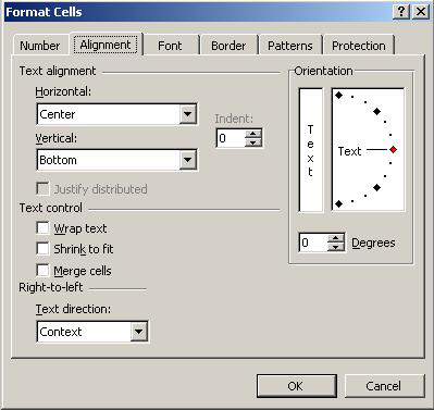
Now use the Orientation section of this menu to alter the direction of the text in your cells - The orientation of the text won’t change until you click on OK.

I very rarely use this feature of Excel, but it can be a useful way to save space if you have long column headers.

Text Control

‘Wrap text’ and ‘Shrink to fit’ are very useful feature that can be used to help keeps your spreadsheet from looking messy. If you have to include a lot of information in one cell, but you don’t want to have a really wide column you can use one of these features.

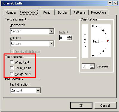
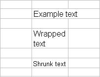
Personally I find ‘Wrap text’ to be the more useful of these 2 features, but it’s worth remembering that ‘Shrink text’ exists as you may sometimes find it helpful.

Merge Cells

This is a great little feature of Excel that can help you to lay out your spreadsheets in a way that is easy to follow - Essentially is allows you to combine several cells into one single, larger cell. You can find the 'Merge cells' button on the Formatting toolbar:

‘Merge cells’ will allow you to combine a series of connected cells across rows and columns – I've used it in our example to center the title. The centering is a by-product of merging the cells, but if you don’t want the contents to be centered you can always realign them as described earlier on.

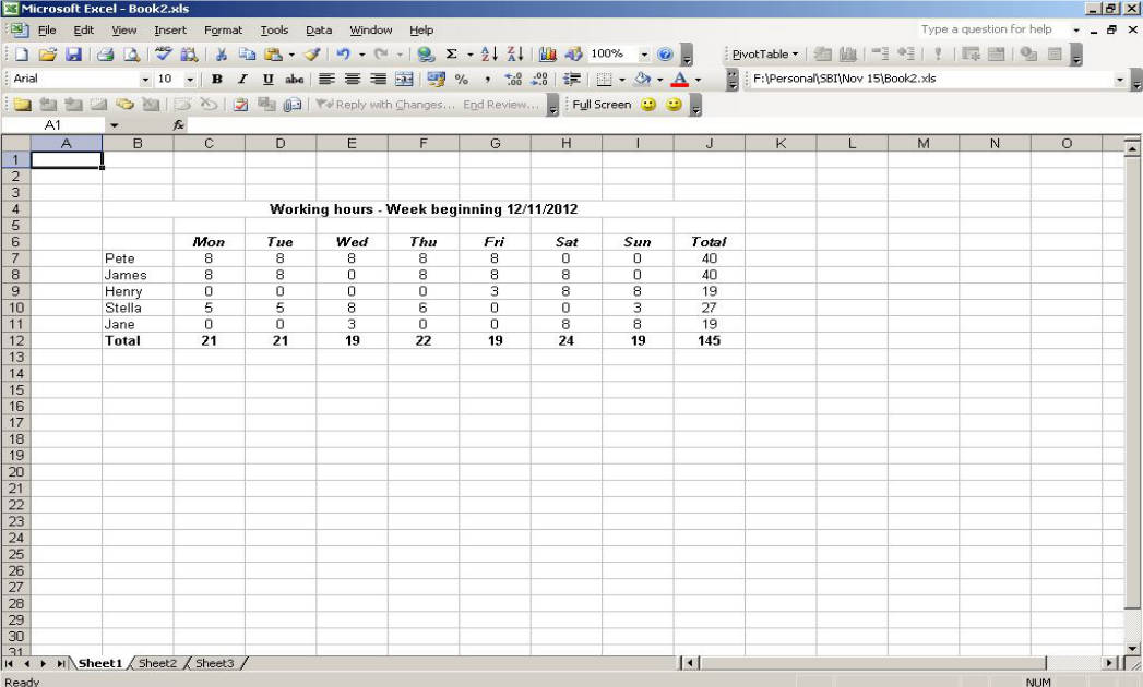
I’d suggest that you take a few moments to have a play with this feature and get used to it – It won’t be useful every day but it’s worth remembering for future use.

Borders

Adding borders to your data is often necessary to ensure that it’s easy for other people to understand. To add borders you’ll need to highlight the cells you want to include, then right click and select ‘Format Cells’. In the resulting menu you’ll want to select the ‘Border’ tab, and you’ll be confronted with a menu that looks like this:

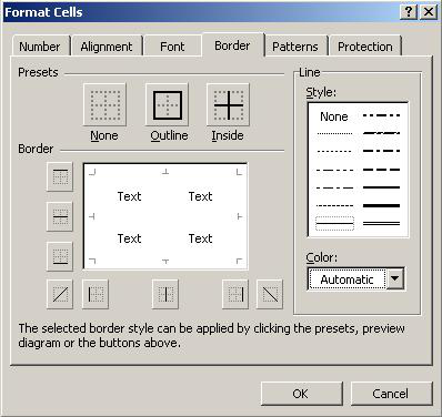
I suggest that you play around with this for a few moments as you’ll see that you have dozens of options for line styles, thicknesses, colours, etc. You can also choose which parts of your selection you want to border.

As a general rule, less is more. Sometimes it’s useful to include bold borders, etc. but for the most part I’d suggest you keep it simple. If you aren’t sure then simply selecting the default line width and applying it to the outline and inside of your selection is always a reasonable option. In the case of our example it would look like this:

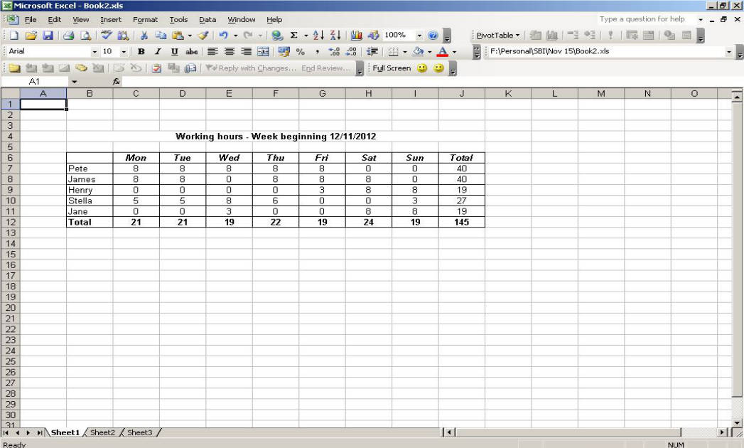
This is a fairly clear way to present the data, but I prefer to be a bit more minimalist. I arranged my borders like this:

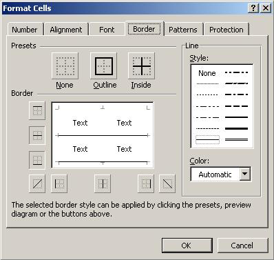
Which in turn makes our example data look like this:

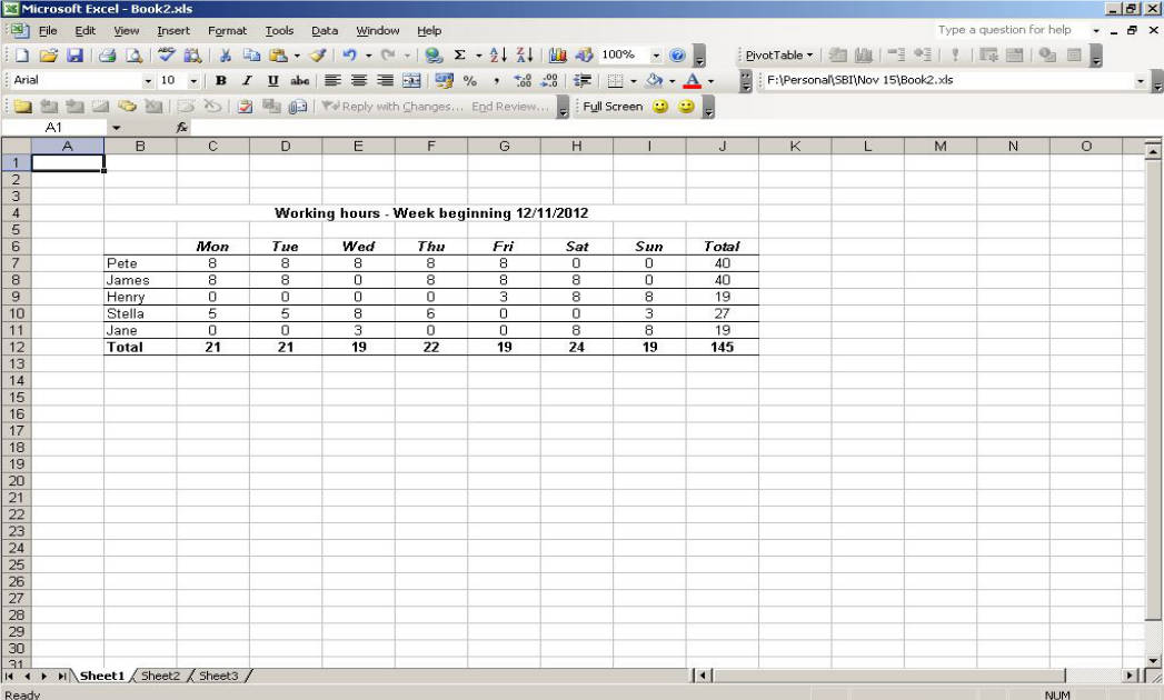
With experience you’ll find that you have a preference for certain border styles, which is great – Just try to keep it simple!

Shading

Adding background colours to some of your cells is another way to help other people to understand your spreadsheets, but again it’s important to use it lightly. Adding some gentle colour to important areas of a spreadsheet can be beneficial, just be careful not to go overboard.

To add colours just select the cells you want to add shading to, right click and select ‘Format Cells’. In the resulting menu you’ll need to select the ‘Patterns’ tab, and you’ll see a menu that looks like this:

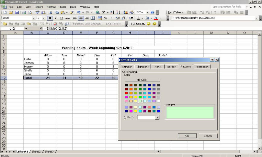
If you click on the drop-down arrow labelled ‘Pattern’ you’ll find that can also add a texture to your selection. Now just select the background color you want and click OK. Now our example table is finished, and it looks like this:

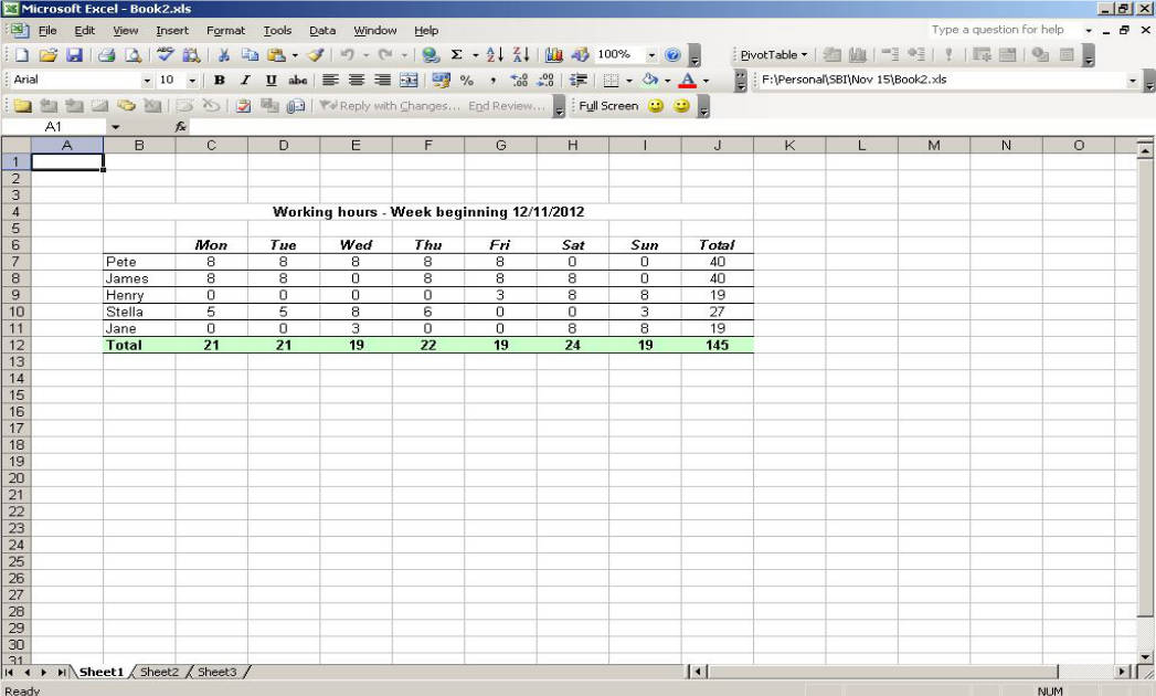
Much easier to understand than the unformatted data we started with, wouldn't you say? It only takes a few moments to format data in a way that makes it easier to understand.

Inserting columns and rows

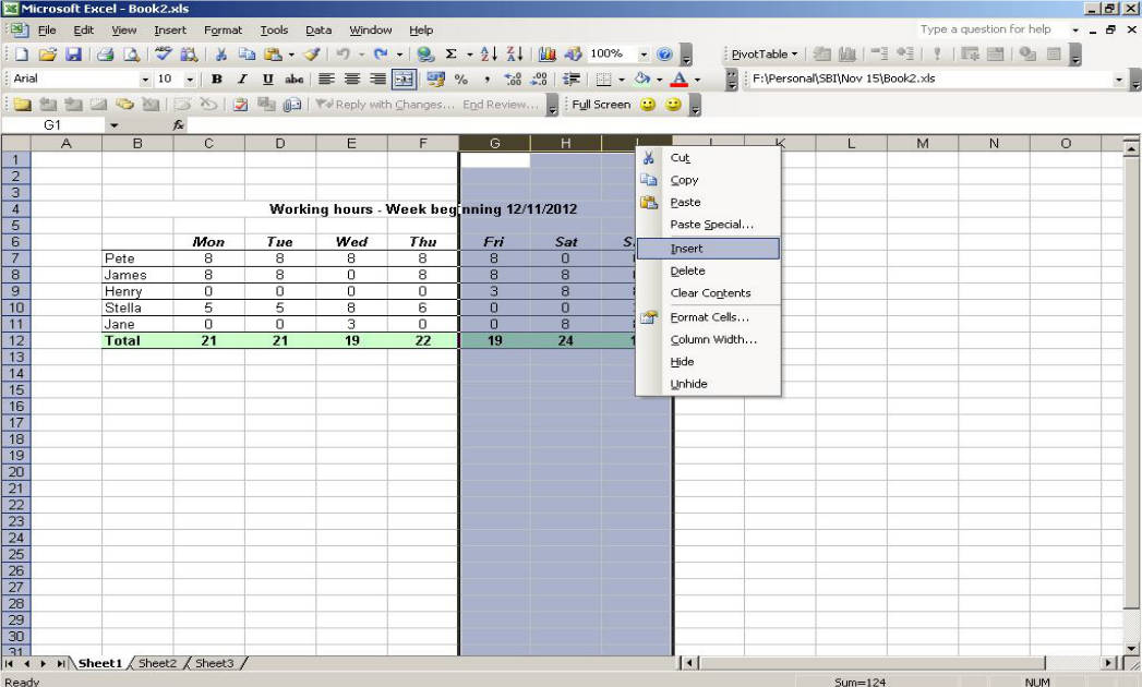
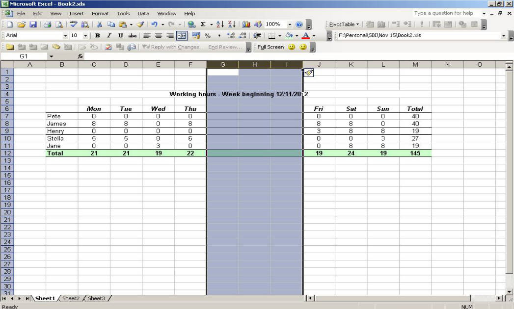
You’ll often find it necessary to insert columns and rows into spreadsheets that you’ve already created. In order to do this, you can simply right click on a column or row label and select ‘Insert’ – This will add a new column or row before the one you’ve clicked on. You can use this same process to add multiple rows or columns by selecting several, right clicking and selecting ‘Insert’. This will add as many columns or rows as you have highlighted before the first row or column in your selection.

Before:

After:

So that’s all for this Formatting in Excel Tutorial, I hope you’ve found it helpful. Please let me know your thoughts by completing the feedback form at the bottom of the page.

Looking for more? Return to Excel Tutorials or the Office Software homepage

This Form cannot be submitted until the missing fields (labelled below in red) have been filled in
Let me know what you think:
Please note that all fields followed by an asterisk must be filled in.
First Name*
E-Mail Address*
Feedback*
Please enter the word that you see below.